The principle of Helmholtz reciprocity – which states that conjugate optical processes, such as swapping the source and the detector in EM, produce equivalent results – can be used to relate HRTEM and STEM imaging modalities. Specifically, virtual images formed by single BF pixels in a STEM detector are equivalent to HRTEM images with planewave illumination tilted to the BF pixel angle. By extension an annular BF detector, which sums multiple BF pixels, is equivalent to an incoherent integral of tilted HRTEM images over the range of angles inside the BF detector.

Further, when the incoming illumination is aberrated, features in these tilted virtual BF images experience lateral shifts proportional to the gradient of the aberration surface and the tilted illumination angle. Tilt-corrected BF STEM (tcBF) Yu et al., 2024, also known as parallax imaging Varnavides et al., 2024, utilizes this fact to computationally align all of the tilted vBF images to the optic axis. Summing over the these aligned vBF images, yields a much sharper, coherent BF image.

Tilt-Corrected BF STEM CTF¶

The tcBF CTF can be understood by starting with the complex-valued aperture overlap function (2.11), reproduced here for convenience:

To proceed, we wish to factorize out the part containing the lateral shifts needed to align the tilted vBF images from (5.1). The remaining terms we collect into a function $\Beta(\bm{q},\bm{k})$ such that we obtain:

Here, the term involving the gradient of the aberration surface, $\nabla \chi$, is a phase ramp corresponding to the lateral shifts observed in tcBF measurements.

Since, in traditional tcBF processing, these lateral shifts are simply used to align the vBF images, without performing any additional deconvolution, they do not contribute to the tcBF CTF. As such, the tcBF CTF is obtained by summing $\Beta(\bm{q},\bm{k})$ over $\bm{k}$:

which we recognize as the HRTEM CTF modulated by the aperture auto-correlation envelope.

Source:Pixelated Parallax

VBox(children=(HBox(children=(FloatSlider(value=-128.0, description='negative defocus, $C_{1,0}$ [Å]', layout=…

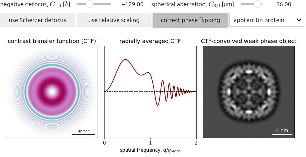
Figure 5.1 plots (5.3) for low-order isotropic aberration coefficients, namely $C_{1,0}$ and $C_{3,0}$. We note the following:

• Similar to HRTEM, the tcBF CTF features zero-crossings and thus contrast reversals. This is often ameliorated using CTF “phase-flipping”.
• Since the tcBF CTF shares the same zero-crossings as HRTEM, the Scherzer defocus is indeed the optimum configuration for an uncorrected microscope.

Low-Order Approximation¶

Equation (5.2) is only satisfied if we approximate the shifted aberration surface $\chi(\bm{q} \pm \bm{k})$ with the first-order term of its Taylor expansion:

where $H_{\chi}(\bm{q})$ is the Hessian of the aberration surface.

Truncating (5.4) after the gradient term yields an exact result when the aberration phase function $\chi(\bm{q})$ is quadratic in $\bm{q}$. This includes terms such as defocus and astigmatism, which are proportional to $q^2$, $q_x^2 - q_y^2$, and $2q_x q_y$. For such quadratic forms, the Hessian is constant and thus the second-order error term becomes independent of $\bm{q}$, contributing only a global, physically irrelevant phase shift in (5.2). However, for higher-order aberration coefficients, such as coma and spherical aberration, (5.2) introduces non-trivial approximation errors which scale with $\bm{q}$ and increase for larger $\bm{k}$ support, reflecting the non-linear curvature of the aberration surface.